
SOLUTION
-
The Kalman Filter: In Theory
-
The Kalman Filter: In Action (MATLAB)
-
MATLAB Simulink

The Kalman Filter in theory
THE KALMAN FILTER
An In-Depth Explanation
The Basics
-
Supports estimations of past, present, and even future states.
-
Minimizes the variance of the estimation error by reducing noise.
-
Can be used to
-
estimate a moving vehicles position
-
Kalman Filter uses a recursive method by making estimates
over and over again


The Equation
-
It consists of three equations, each involving matrix manipulation.
-
The T superscript indicates matrix transposition.
-
The K matrix is called the Kalman gain
-
The P matrix is called the estimation error covariance
-
X is the state estimate
Steady-State Kalman Filter code


Steady-State Kalman Filter Output

A Kalman Filter Application: Vehicle Location Estimation

First, simplify the equation if possible:
Equation 1 can be simplified by removing the process noise as the gps used for this example effectively reduces the noise to 0. similarly we are able to remove the control matrix and variable can be removed
How does this knowledge help?
We can extrapolate the vehicle time state for n+1 and describe with the following system of equations and matrix.

{

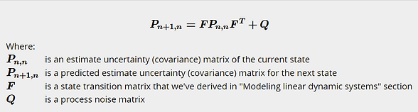
Equation 2: Covariance Extrapolation Equation
Much like the name suggests, equation 2's sole purpose is to find the covariance in the state equations Estimations.
How the Equation is used:
First, we will find the estimate uncertainty in matrix form:

We can safely assume that X and Y estimate errors are independent from one another. Therefore,we disregard mutual terms.

Next, we will find the process noise matrix:

Once again we assume that X and Y estimate errors are independent from one another. Therefore,we disregard mutual terms.

Using the derivation for a constant acceleration motion model we find the following matrix where:
-
Change in T is the time between successive measurements
-
sigma random variance in the estimations

Now we can plug our blocks into the covariance extrapolation equation
*To save space, we have not included the equation, only the solution. The aid of a tool like Matlab is vital.

We can safely assume that X and Y estimate errors are independent from one another. Therefore,we disregard mutual terms.
Equation 3/4: The measurement Equation & Uncertainty

The measurement provides the x,y location of the vehicle while the uncertainty measures covariance.
Note for this example we do not use the random noise vector present in the equation.
How the Equation is used:


The random noise vector is ignored for the sake of this example because it comes from the enviroment.
Z is distinguished by the planes of the example
H is then solved for considering the measurable states necessary for the problem.
The measurement uncertainty:

X and Y estimate errors are independent from one another. Therefore, we disregard mutual terms.

Measurement uncertainty, m in the matrix is usually measured through the environment around sensors, for this example it will be ignored
Equation 5: The Kalman Gain

When solving for the kalman gain we are looking to solve for a gain the minimizes estimate variance
How the Equation is used:
As we now have all of the blocks necessary, we use a matrix calculator to solve for our answer

Kalman gain
Equation 6/7: The State/Covariance update equations


Similar to the Equation 1 and 2 however as the name suggests these equations update the state and covariance as the filter runs
How the Equation is used:
Note that all of the Blocks necessary for these two equations are from previous steps.

Now that we have previously discussed the workings of a basic Kalman filter, we can work through a problem more applicable to the project at hand.
For This Example a vehicle has sensors for its XY location and we will assume that all acceleration will be smooth and constant.
Equations Necessary:
Equation 1: State Extrapolation Equation
Using Equation 1, we can predict the next system state, based on the knowledge of the current state. It extrapolates state vector from the present (time step n) to the future (time step n+1).
How the Equation is used:
Next, find the state vector:

In this example, the car we are making state estimates can be described by the state vector X describing the velocity, acceleration and position of the car in the x,y plane.
n