The Extended Kalman Filter via MATLAB

i.e. The Kalman Filter in action

OR

Motion Generation(Random)

Random Motion Block

Random Motion Block:

This Simulink block creates a random motion signal the parameters are as follows:

Noise power: The variance in the generated signal.

Sample Time: How often the generated signal is sampled.

Seed: Each set of random motion is defined by a seed value, the random motion we used is defined with [23341].

Motion to acceleration cluster

Acceleration to Simulink

Acceleration Cluster:

This cluster of blocks creates the acceleration data from the motion through integration, applies a gain of one to that value, and then steps the random motion forward once while porting the acceleration data to the rest of the Simulink.

Motion Generation(Measured)

From Workspace block:

Unlike the way the Random motion block creates a random set of motion, the from workspace block looks at a Data struct created in the workspace that describes the XY acceleration data and time data that was measured using the matlab mobile app.

From Workspace block Parameters:

Data: Data refers to whatever data is being read from in the workspace, in this case it is the wave struct containing the measured acceleration data.

Output data type: Refers to the data type of the output from the struct, in this case we use the option for inheriting the type of the struct.

Sample time: The sample time for the data.

Interpolate data: Used to fill in data that is unknown, as we are making a kalman filter for estimation, we do not want this on.

Enable zero-crossing detection: Dynamically effects time-step to decrease run time.

Form output after final data value: Form the data resorts to after data is exhausted if run time exceeds data.

*Pictured below is the acceleration data used for the measured example and a snip of Matlab mobile*

To Velocity and Position Block:

Integrator blocks for acceleration and position:

Through these integrator blocks the acceleration data(that from now on refers to both the random and measured data) is integrated into its velocity and position values

CTP and Measurment noise cluster:

Measurement noise:

The measurement noise block replicates the natural random noise vector that can be found in all Kalman filters due to the environments in which they operate

CTP blocks:

The Cartesian to polar block changes the coordinate system to polar as it is better implemented in the Extended Kalman filter

Addition blocks:

The addition block adds the measurement noise to the range and bearing signals

Measurement noise block Parameters:

Mean: Specifies the mean of the random numbers

Variance: Refers to the intensity of noise.

Seed: Each set of random motion is defined by a seed value, the random motion we used is defined with [0].

Sample time: How often the random noise is measured

Ext-Kalman and DT block cluster:

Ext-Kalman and DT block input/output:

Meas: The measurements for bearing and range are input into the Extended Kalman filter block.

dt: Implies the state estimations are sampled at a rate of .1 seconds.

xhatOut: The estimated output of each of the inputs after being processed through the Kalman Filter.

ExtKalman Code Explained

Initialization

To get the Kalman Filter started, we need to initialize some things,

xhat is initializing the starting point of each of the estimations
P is creating a 4x4 matrix filled with zeros
Q and R is the covariance of the output noise

Jacobians

The above equation shows that the position changes by dt times the velocity over a short period of time and that the velocity remains constant in both x and y directions.
yhat is the differentiation of a trigonometric identity and Hk is the Jacobian for the measurement equation.
The range and bearing are related to the x and y displacements by the equations

Propagation

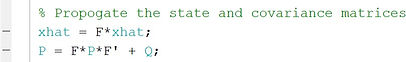
These equations are responsible for making the predictions, where

k denotes a discrete point in time (with k-1 being the immediate past time point)
uk is a vector of inputs
xk is a vector of the actual states, which may be observable but not measured

Kalman gain and updating the state and covariance estimates

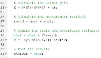
These equations give the corrector step, where

Pk is an estimate of the covariance of the measurement error
Kk is the Kalman gain
xhat is the current estimate of the states

Finally The estimates are sent out to the Kalman Filter

Simulink & Matlab

Simulink is the Mathworks developed platform for Model-Based Design that supports system-level design, simulation, automatic code generation, and continuous test and verification of embedded systems that pair with the Matlabs.

For this project we used Matlab & simulink together to simulate a simple Kalman filter recieving and perform state estimations on positon and velocity vectors through randomly generated and physically measured acceleration data.

Simulink

First we will take a look at how we use Simulink to simulate a system with a Kalman filter.

As spoken about above will look at two different systems, one with an artificial acceleration data, and one with data gathered on a roughly 10 minute drive

Extended Kalman system Simulink walkthrough

*Note*

This examination will not look at the bottom path as it is only used to port information to the scopes for viewing.

*Note*

The only difference in the random and measured acceleration Simulinks is the first block. This will be covered.

Extended Kalman Filter Outputs

Simulink Random Acceleration Output

X-position and Y-Position outputs

When considering the outputs of the extended Kalman filter it is important to remember the frame of reference that the positions are being calculated in.

If we consider the map to the right we find that the observation point calculates the

X-Displacement away from the train station and the amount of Y-Displacement in both the negative and positive directions.

Now looking at the output for the extended Kalman Filter, we find a similar "map". However now the reference point is located in the first second of the Xpos and Ypos signals.

X

Y

X-Velocity and Y-Velocity outputs

I'm a paragraph. Click here to add your own text and edit me. It's easy.

The X and Y velocities are intuitive and should be referenced as normal velocities.

Measured Acceleration Output

Unfortunately the method in which we recorded the acceleration data from a car ride has some shortcomings. Because of the iPhones frame of reference, it only records X-acceleration. You can inspect this Output in the same way as the last randomly generated output, but for the sake of the project we will refer to the randomly generated Outputs as the ideal input to our Simulink.

Interpretations & Conclusion

What did we learn?

Operations of a GPS
Applications of DSP to approximation of unknown states
Applications of DSP to the system design of a GPS receiver
The Basic Kalman Filter
The Extended Kalman Filter
The uses of MATLAB Simulink
Relation to GPS approximation

Where can we take this project next?

Move the MATLAB Simulink Model to Xilinx Vivado and then to an FPGA
"Zoom out" and now focus on developing an efficient GPS receiver by optimizing the parameters of a basic receiver to the specifications and needs of our Kalman filter or vice versa
"Zoom out" more and implement the Kalman filter in an android application for train departure and arrival times